A discrete Gibbs random field (GRF) is specified by a probability mass function of the image as follows:

where  is the energy function, and
  , over all
 images; G being the number of gray levels, and the image is
of size
  . Except in very special
circumstances, it is not feasible to compute Z. A relaxation-type
algorithm described in [14] simulates a Markov chain through an
iterative procedure that re-adjusts the gray levels at pixel locations
during each iteration. This algorithm sequentially initializes the
value of each pixel using a uniform distribution. Then a single pixel
location is selected at random, and using the conditional distribution
that describes the Markov chain, the new gray level at that location
is selected, dependent only upon the gray levels of the pixels in its
local neighborhood. The sequential algorithm terminates after a given
number of iterations.

The sequential algorithm to generate a Gibbs random field described in [14] and [17] are used as a basis for our parallel algorithm. We introduce some terminology before presenting the parallel algorithm.
The neighborhood model N of a pixel is shown in
Figure 4. For all the algorithms given in this paper, we
use a symmetric neighborhood  which is half the size of N.
This implies that if the vector
  , then
 , but only one of
  is in
is in  . Each element of array
  is taken to represent the parameter associated with its corresponding
element in
  . We use the notation
  to represent the
gray level of the image at pixel location
  .
.
Our Gibbs random field is generated using a simulated annealing type
process. For an image with G gray levels, the probability  is binomial with parameter
  , and number of trials G-1. The array
{T} is given in the following equation for a first-order model:
and is a weighted sum of neighboring pixels at each pixel location. Additional examples of {T} for higher order models may be found in [14].
This algorithm is ideal for parallelization. The calculation of {T} requires uniform communications between local processing elements, and all other operations needed in the algorithm are data independent, uniform at each pixel location, scalable, and simple. The parallel algorithm is as follows:

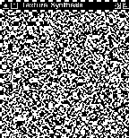
Figure: Isotropic Inhibition Texture using Gibbs Sampler (Texture 9b from [14]).
An example of a binary synthetic texture generated by the Gibbs Sampler is given in Figure 5.
With  processing elements, and within each
iteration, step 2.1 can be executed in O
computational steps and O communication
complexity, and steps 2.3 and 2.4 in O
computational time, yielding a computation complexity of

and communication complexity of

per iteration for a problem size of  .
.
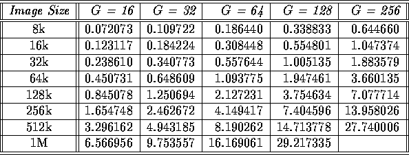
Table 1 shows the timings of a binary Gibbs sampler for model orders 1, 2, and 4, on the CM-2, and Table 2 shows the corresponding timings for the CM-5. Table 3 presents the timings on the CM-2 for a Gibbs sampler with fixed model order 4, but varies the number of gray levels, G. Table 4 gives the corresponding timings on the CM-5.

Table 1: Gibbs Sampler timings for a binary (G = 2) image (execution time in seconds per iteration on a CM-2 running at 7.00 MHz)

Table 2: Gibbs Sampler timings for a binary (G = 2) image (execution time in seconds per iteration on a CM-5 with vector units)

Table 3: Gibbs Sampler timings using the 4th order model and varying G (execution time in seconds per iteration on a 16k CM-2 running at 7.00 MHz)

Table 4: Gibbs Sampler timings using the 4th order model and varying G (execution time in seconds per iteration on a 32 node CM-5 with vector units)