We introduce the following approach as an improved method for estimating GMRF parameters of textured images. The method of maximum likelihood gives a better estimate of the texture parameters, since the asymptotic variance of the MLE is lower than that of the LSE. We also show a much faster algorithm for optimizing the joint probability density function which is an extension of the Newton-Raphson method and is also highly parallelizable.
Assuming a toroidal lattice representation for the image
 and Gaussian structure for noise sequence
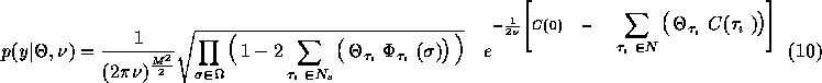
 , the joint probability density function is the
following:
, the joint probability density function is the
following:
In (10),  is the sample correlation estimate at
lag
is the sample correlation estimate at
lag  . As described in [2] and [3],
the log-likelihood function can be maximized: (Note that
. As described in [2] and [3],
the log-likelihood function can be maximized: (Note that 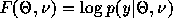 ).
).


For a square image,  is given as follows:

This non-linear function F is maximized by using an extension of
the Newton-Raphson method. This new method first generates a
search direction  by solving the system

Note that this method works well when  is a symmetric,
positive-definite Hessian matrix. We then maximize the step in
the search direction, yielding an approximation to
is a symmetric,
positive-definite Hessian matrix. We then maximize the step in
the search direction, yielding an approximation to  which
attains the local maximum of
which
attains the local maximum of  and
also satisfies the constraints that each of the
and
also satisfies the constraints that each of the  values in the
logarithm term for F is positive. Finally, an optimality
test is performed. We set
values in the
logarithm term for F is positive. Finally, an optimality
test is performed. We set  , and if
  is sufficiently close to
  ,
the procedure terminates. We give the first and second derivatives of
F with respect to
,
the procedure terminates. We give the first and second derivatives of
F with respect to  and
and  in
[1].
in
[1].
For a rapid convergence of the Newton-Raphson method, it must be
initialized with a good estimate of parameters close to the global
maximum. We use the least squares estimate given in
Subsection 3.1 as  , the starting value of the
parameters.
, the starting value of the
parameters.
In Figure 5, we show the synthesis using least squares and maximum likelihood estimates for tree bark obtained from standard textures library. Table 2 shows the respective parameters for both the LSE and MLE and give their log-likelihood function values. This example shows that the maximum likelihood estimate improves the parameterization. In addition, CM-5 timings for these estimates varying machine size, image size, and neighborhood models can be found in Figure 6 for both fourth and higher order models on this selection of real world textured images. The value plotted is the mean time over thirteen diverse images, and errors bars give the standard deviation. More explicit tables, as well as CM-2 timings, for these estimates can be found in [1].