 , then
The input sets are defined as follows. If the set's tag ends with 8,
16, 32, 64, or 128, there are initially 8192, 16384,
32768, 65536, or 131072 elements per processor, respectively.
The values of these elements are chosen by the method represented by
the first letter. If the total number of elements per processor is
q, and the processor is labeled j, for  , then
 ;
;
 ;
;
 .
.
 Landsat TM image)
contains a total of
  elements, which is the same size as the
input sets ending with tag 8 on a 32 processor machine. Set L1024,
with a total of
  elements, is derived from a similar
  image, and has the same number of elements as an input
set ending with tag 32 on a 32 processor machine.
On the SP-2, results given in Figure 7 are only for Method B, with each timing bar broken into two partitions showing the portion of the total running time spent performing data redistribution versus the remaining selection time. As these empirical data show, dynamic data redistribution is only a small fraction of the total running time, which implies that the data is fairly balanced after each iteration. Also, in every case, Method B outperforms Method A.

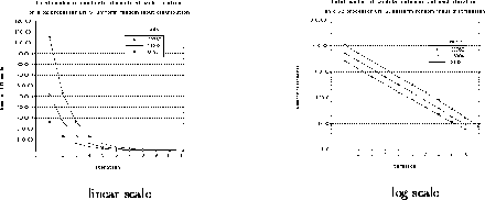
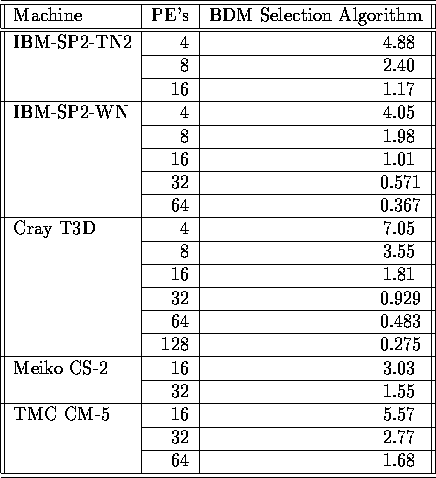
Figure 8: Number of candidates per iteration
We benchmark our selection algorithm in Table I.
The input for this problem, taken from the NAS Parallel Benchmark for
Integer Sorting [5], is  integers in the range
 , spread out evenly across the processors. Each key is the
average of four consecutive uniformly distributed pseudo-random
numbers generated by the following recurrence:

where  and the seed
  . Thus, the
distribution of the key values is Gaussian. On a p-processor
machine, the first
  generated keys are assigned to
  ,
the next
  to
to  , and so forth, until each processor
has
  keys.
keys.

Table I: Execution Times for the High-Level BDM Selection (in seconds)
on the NAS IS input set
The empirical results presented in Table I clearly
show that the selection algorithm is scalable with respect to machine
size, since doubling the number of processors solves the problem in
about half the time. This is consistent with the BDM analysis given in
Eq. (7). For  and machine sizes typically
in the order of tens or hundreds of processors, computation dominates
the selection algorithm, and execution time scales as
  .
(For verification, the median of the NAS input set is 262198.) Our
code for selection, written in the high-level parallel language of
SPLIT-C , is ported to the parallel machines with absolutely no
modifications to the source code. Even without machine-specific
(low-level) code optimizations that are typically needed for superior
parallel performance, we have an algorithm which performs extremely
well across a variety of current parallel machines such as the Cray
T3D, IBM SP-2, TMC CM-5, and Meiko CS-2.
Next we compare our selection algorithm to that of the trivial method of selection by parallel integer sorting on the TMC CM-5. As shown in Table II, our high-level selection algorithm beats the fastest sorting results for the NAS input that are known to the authors. Note that the algorithm in [6] is machine-specific and does not actually result in a sorted list.

Table II: Execution Time for Selection on a 32-processor CM-5 on the
NAS IS input set
Figure 8 shows that the parallel selection algorithm
for R8, R16, and R32, reduces the candidate elements by
approximately one-half during each successive iteration. In this plot,
p=32; thus, when the data sets shrinks to a size less than  ,
i.e. smaller than 1024, a sequential algorithm is employed to solve
the corresponding selection problem.