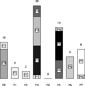
Figure 2: Example of Dynamic Data Redistribution (Method A) with p=8 and n=63

Figure 2: Example of Dynamic Data Redistribution (Method A) with p=8 and n=63
A simple method for dynamic data redistribution ranks each element in
order across the p processors, and assigns each set of q
consecutively labeled elements to a processor, where  . Note that when p does not
divide n evenly, the last processor will receive less than q
elements. We refer to this as Method A.
Figure 2 shows a dynamic data redistribution example for
Method A. This is a simple example for 8 processors and 63
elements, with an arbitrary initial distribution of  . Here,
  , for
, for  , while
  , since
  receives the remainder of elements when p does not divide the total
number of elements evenly.
An algorithm for Method A first calls the
CONCAT communication primitive and assigns it to array
 , a
, a  shared array. Another
  shared
array of prefix-sums of the values from N, say PS, is derived from
 by simple local running sum calculations. Thus, every
processor contains local copies of all prefix-sums. Suppose elements
are logically ranked in consecutive order from 1 to n. In the
final layout, processor i will hold elements ranked from q i + 1
to
  , inclusively. Using the prefix-sum information, each
processor easily determines where these elements are located and
issues READ primitives for the respective remote locations to
fill the
  distributed
output array.
The analysis for the dynamic data redistribution algorithm using the
BDM model is as follows. The CONCAT primitive requires
communication  and
and  (Eq. (2)). The local prefix-sum calculation
requires O
 . Determining the location of elements to be read
using the prefix-sums has computational complexity of
  . Assume that the maximum number of elements initially on a processor
is m, i.e.,
  . The READ primitive for
actually issuing the remote read requests uses
  and
and  since each processor fetches at most
  elements, but in the worst case, a processor
is the source of m fetched elements. Since these requests are
pipelined, only a single latency
  is incurred. Since
  , the dynamic data redistribution algorithm has the
following complexity:
Note that the input distribution N for dynamic data redistribution
can range from already balanced data  to the
case where all data is located on a single processor
  . For a large class of
irregular problems such that data are distributed with a certain class
of distributions, it has been shown that the distribution is typically
closer to the first scenario,
  [28].
[28].