The design of communication efficient parallel algorithms depends
on the existence of efficient schemes for handling frequently
occurring transformations on data layouts. In this section,
we consider data layouts that
can be specified by a two-dimensional array A, say of size
 , where column i of A contains a subarray
stored in the local memory of processor
, where column i of A contains a subarray
stored in the local memory of processor  , where
 . A transformation
  on the layout A will
map the elements of A into the layout
on the layout A will
map the elements of A into the layout  not necessarily
of the same size. We present optimal or near optimal
algorithms to handle several such transformations including
broadcasting operations, matrix transposition, and
data permutation. All the algorithms described are deterministic except
for the algorithm to perform a general permutation.
not necessarily
of the same size. We present optimal or near optimal
algorithms to handle several such transformations including
broadcasting operations, matrix transposition, and
data permutation. All the algorithms described are deterministic except
for the algorithm to perform a general permutation.
We start by addressing several broadcasting operations. The simplest
case is to broadcast a single item to a number of remote locations. Hence
the layout A can be described as a one-dimensional array and we assume
that the element  has to be copied into the remaining entries of
A. This can be viewed as a concurrent read operation from
location
has to be copied into the remaining entries of
A. This can be viewed as a concurrent read operation from
location  executed
by processors
executed
by processors  .
The next lemma provides a simple algorithm to solve this problem; we
later use this algorithm to derive an optimal broadcasting algorithm.
.
The next lemma provides a simple algorithm to solve this problem; we
later use this algorithm to derive an optimal broadcasting algorithm.

Proof: A simple algorithm consists of p-1 rounds that can be pipelined.
During the rth round, each processor  reads
reads  , for
, for  ; however,
only
; however,
only  is copied into A[j].
Since these rounds can be realized with p-1 pipelined prefetch read operations, the
resulting communication complexity is
is copied into A[j].
Since these rounds can be realized with p-1 pipelined prefetch read operations, the
resulting communication complexity is  .
.

We are now ready for the following theorem
that essentially establishes the fact that a k-ary balanced tree
broadcasting algorithm is the best possible for  (recall that we
earlier made the assumption that
(recall that we
earlier made the assumption that  is an integral multiple of m).
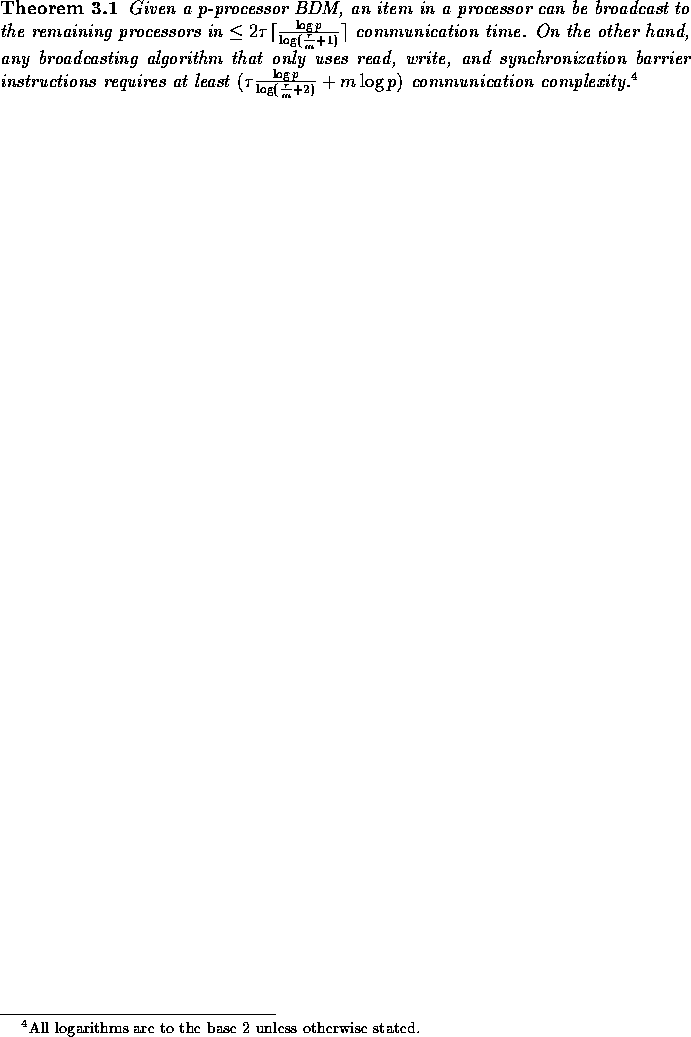
Proof: We start by describing the algorithm.
Let k be an integer to be determined later. The algorithm
can be viewed as a k-ary tree rooted at location  ; there
are
; there
are  rounds. During the first round,
 is broadcast to locations
  , using the
algorithm described in Lemma 3.1,
followed by a synchronization barrier. Then during the second round,
each element in locations
, using the
algorithm described in Lemma 3.1,
followed by a synchronization barrier. Then during the second round,
each element in locations  is broadcast
to a distinct set of k-1 locations, and so on. The communication
cost incurred during each round is given by
is broadcast
to a distinct set of k-1 locations, and so on. The communication
cost incurred during each round is given by  (Lemma 3.1). Therefore the total communication cost is
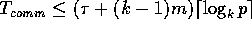 . If we set
 , then
 .
.
We next establish the lower bound stated in the theorem.
Any broadcasting algorithm using only read, write, and
synchronization barrier instructions can be viewed as operating in phases, where
each phase ends with a synchronization barrier (whenever there are more
than a single phase). Suppose there are s phases.
The amount of communication to execute
phase i is at least  , where
  is the maximum number of
copies read from any processor during phase i. Hence the total amount of
communication required is at least
is the maximum number of
copies read from any processor during phase i. Hence the total amount of
communication required is at least  .
Note that by the end of phase i, the desired item has reached at most
.
Note that by the end of phase i, the desired item has reached at most
 remote locations.
It follows that, if by the end of phase s, the desired item has reached all
the processors, we must have
remote locations.
It follows that, if by the end of phase s, the desired item has reached all
the processors, we must have  .
The communication time
.
The communication time  is minimized when
  , and hence
  .
Therefore
.
Therefore  and the communication time is
at least
and the communication time is
at least  .
We complete the proof of this theorem by proving the following claim.
.
We complete the proof of this theorem by proving the following claim.
Claim:
 , for any
  .
.
Proof of the Claim: Let  ,
,
 ,
,  ,
and
,
and  . Then,

(Case 1) ( ): Since
  is decreasing and
  is increasing in this range, the claims follows easily by noting that
 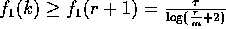 and
and 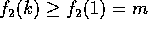 .
.
(Case 2) (k>r+1): We show that  is increasing when k>r+1
by showing that
is increasing when k>r+1
by showing that  for all integers
  . Note that since
 , we have that
  is at least
as large as
is at least
as large as  which is positive for all nonzero
integer values of k. Hence
which is positive for all nonzero
integer values of k. Hence 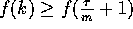 and the claim follows.
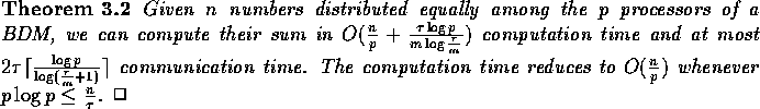
The sum of p elements on a p-processor BDM can be computed in at most
 communication time by
using a similar strategy.
Based on this observation, it is easy to show the following theorem.
communication time by
using a similar strategy.
Based on this observation, it is easy to show the following theorem.
Another simple broadcasting operation is when each processor has to broadcast
an item to all the remaining processors. This operation can be executed in
 communication time as shown
in the next lemma.
communication time as shown
in the next lemma.

Proof:
The bound of  follows from the simple
algorithm described in Lemma 3.1.
If p is significantly larger than m,
then we can use the following strategy.
We use the previous algorithm until each processor has m elements.
Next, each block of m elements is broadcast in a circular fashion
to the appropriate
follows from the simple
algorithm described in Lemma 3.1.
If p is significantly larger than m,
then we can use the following strategy.
We use the previous algorithm until each processor has m elements.
Next, each block of m elements is broadcast in a circular fashion
to the appropriate  processors.
One can verify that the resulting communication complexity is
processors.
One can verify that the resulting communication complexity is  .
.

Our next data movement operation is the
matrix transposition that can be defined as follows. Let  and
let p divide q evenly without loss of generality. The
data layout described by A is supposed to be rearranged into
the layout
and
let p divide q evenly without loss of generality. The
data layout described by A is supposed to be rearranged into
the layout  so
that the first column of
so
that the first column of  contains the first
  consecutive rows of A
laid out in row major order form,
the second column of
consecutive rows of A
laid out in row major order form,
the second column of  contains the second set of
  consecutive rows of A, and so on. Clearly, if q=p, this corresponds
to the usual notion of matrix transpose.
consecutive rows of A, and so on. Clearly, if q=p, this corresponds
to the usual notion of matrix transpose.
An efficient algorithm
to perform matrix transposition on the BDM model is similar
to the algorithm reported in [8]. There are p-1 rounds that can be
fully pipelined by using prefetch read
operations. During the first round, the appropriate
block of  elements in the ith column of A is read by processor
 into
the appropriate locations,
for
into
the appropriate locations,
for  . During the second round, the appropriate block of data
in column i is read by processor
. During the second round, the appropriate block of data
in column i is read by processor  , and so on.
The resulting total communication time is given by
, and so on.
The resulting total communication time is given by
 and the amount of local computation is
  .
Clearly this algorithm is optimal whenever pm divides q. Hence we have
the following lemma.
.
Clearly this algorithm is optimal whenever pm divides q. Hence we have
the following lemma.

We next discuss the broadcasting operation of a block of n elements residing on a single processor to p processors. We describe two algorithms, the first is suitable when the number n of elements is relatively small, and the second is more suitable for large values of n. Both algorithms are based on circular data movement as used in the matrix transposition algorithm. The details are given in the proof of the next theorem.
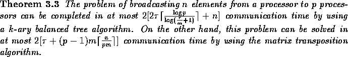
Proof: For the first algorithm,
we use a k-ary tree as in the single item broadcasting algorithm
described in Theorem 3.1, where  .
Using the matrix transposition strategy, distribute the n elements to be broadcast
among k processors, where each processor receives a contiguous block of
size
.
Using the matrix transposition strategy, distribute the n elements to be broadcast
among k processors, where each processor receives a contiguous block of
size  . We now view the p processors as partitioned into k groups,
where each group includes exactly one of the processors that contains a block of
the items to be broadcast. The procedure is repeated within each group and so on.
A similar reverse process can gradually read all the n items into each processor.
Each forward or backward phase is carried out by using the cyclic data movement of
the matrix transposition algorithm. One can check that the communication time can
be bounded as follows.
. We now view the p processors as partitioned into k groups,
where each group includes exactly one of the processors that contains a block of
the items to be broadcast. The procedure is repeated within each group and so on.
A similar reverse process can gradually read all the n items into each processor.
Each forward or backward phase is carried out by using the cyclic data movement of
the matrix transposition algorithm. One can check that the communication time can
be bounded as follows.
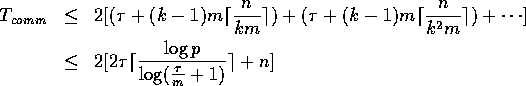
If n>pm, we can broadcast the n elements in
 communication time
using the matrix transposition algorithm of Lemma 3.3 twice, once to
distribute the n elements among the p processors where each processor
receives a block of size
communication time
using the matrix transposition algorithm of Lemma 3.3 twice, once to
distribute the n elements among the p processors where each processor
receives a block of size  , and the second time to circulate these
blocks to all the processors.
, and the second time to circulate these
blocks to all the processors.

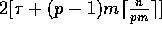
The problem of distributing n elements from a single processor can be solved by using the first half of either of the above two broadcasting algorithms. Hence we have the following corollary.
We finally address the following general routing problem.
Let A be an  array of n elements initially stored
one column per processor in a p-processor BDM machine. Each element of A
consists of a pair (data,i), where i is the index of the processor
to which the data has to be relocated. We assume that at most
array of n elements initially stored
one column per processor in a p-processor BDM machine. Each element of A
consists of a pair (data,i), where i is the index of the processor
to which the data has to be relocated. We assume that at most
 elements have to be routed to any single processor
for some constant
elements have to be routed to any single processor
for some constant  . We describe in what follows a randomized
algorithm that completes the routing in
. We describe in what follows a randomized
algorithm that completes the routing in  communication
time and
communication
time and  computation time, where c is any constant larger
than
computation time, where c is any constant larger
than 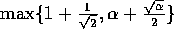 .
The complexity bounds are guaranteed to hold with high
probability, that is, with probability
.
The complexity bounds are guaranteed to hold with high
probability, that is, with probability  , for some
positive constant
, for some
positive constant  , as long as
  ,
where
,
where  is the logarithm to the base e.
The overall idea of the algorithm has been used in various randomized routing algorithms on the mesh. Here we follow more closely the scheme described in [20] for randomized routing on the mesh with bounded queue size.
Before describing our algorithm, we introduce some terminology.
We use an auxiliary array  of size
  for
manipulating the data during the intermediate stages and for holding
the final output, where
for
manipulating the data during the intermediate stages and for holding
the final output, where 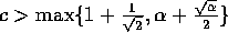 .
Each column of
.
Each column of  will be held in a processor. The array
  can be
divided into p equal size slices, each slice
consisting of
can be
divided into p equal size slices, each slice
consisting of  consecutive rows of
  . Hence a slice contains
a set of
. Hence a slice contains
a set of  consecutive elements from each column and such
a set is referred to as a slot. We are ready to describe our algorithm.
consecutive elements from each column and such
a set is referred to as a slot. We are ready to describe our algorithm.
Algorithm Randomized_Routing
Input: An input array 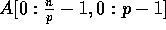 such that each element
of A consists of a pair (data,i), where i is the processor index
to which the data has to be routed. No processor is the destination of
more than
such that each element
of A consists of a pair (data,i), where i is the processor index
to which the data has to be routed. No processor is the destination of
more than  elements for some constant
  .
.
Output: An output array 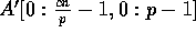 holding the
routed data, where c is any constant larger than
holding the
routed data, where c is any constant larger than
 .
.
begin
 distributes randomly its
  elements into the p slots of the jth column of
  .
.
 so that the jth slice will be stored in
the jth processor, for
so that the jth slice will be stored in
the jth processor, for  .
.
 distributes locally its
 elements such that every element of the form (*,i)
resides in slot i, for
elements such that every element of the form (*,i)
resides in slot i, for  .
.
 (hence the jth
slice of the layout generated at the end of Step 3 now resides in
(hence the jth
slice of the layout generated at the end of Step 3 now resides in  ).
).
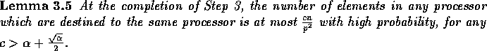
The next two facts will allow us to derive the complexity bounds for our
randomized routing algorithm. For the analysis, we assume that
 .
.

Proof: The procedure performed by each processor is similar to the
experiment of throwing  balls into p bins. Hence the
probability that exactly
balls into p bins. Hence the
probability that exactly  balls are placed in any
particular bin is given by the binomial distribution
balls are placed in any
particular bin is given by the binomial distribution
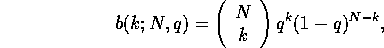
where  ,
,  , and
, and  .
Using the following Chernoff bound for estimating the tail
of the binomial distribution
.
Using the following Chernoff bound for estimating the tail
of the binomial distribution

we obtain that the probability that a particular bin has more than
 balls is upper bounded by

Therefore the probability that any of the bins has more than  balls is bounded by
  and the lemma follows.

Proof: The probability that an element is assigned to the jth slice
by the end of Step 1 is  . Hence the probability that
 elements destined for a single processor fall in the jth
slice is bounded by
elements destined for a single processor fall in the jth
slice is bounded by  since no processor is the destination of more than
  elements. Since there are p slices, the probability that more than
 elements in any processor are destined for the same processor
is bounded by
elements in any processor are destined for the same processor
is bounded by

and hence the lemma follows. 
>From the previous two lemmas, it is easy to show the following theorem.
Remark: Since we are assuming that  , the effect of the
parameter m is dominated by the bound
, the effect of the
parameter m is dominated by the bound  (as
(as  ,
assuming
,
assuming  ).
).
